1 Introduction
March Madness refers to the annual collegiate men’s basketball tournament. The tournament is made up of 64 college teams competing in a single elimination format. In order to win the championship, a team has to win 6 consecutive games. The purpose of this competition/project is to predict the teams’ winning probability of every possible match in the 2018 NCAA men basketball tournament, using the team-level information given before the game was played. For each upcoming game, the predicted result is given by the winning probability of the ‘team 1’ in the game. Most predictors are calculated by the difference between certain variables of team 1 and team 2. Predicting features are calculated, selected, and evaluated in the appropriate ways applied to the models. Prediction accuracy and log-loss are applied for model selection and evaluation
2 Methodology
2.1 Variables Transformation
We analyzed the differences between Team 1 and 2, instead of going through data of each side. Data of AP Poll ranking was transform in a comparable way.
2.2 Variables Selection
There were 4 steps of variables selection, from 56 to 8 for the ultimate model.
2.3 Model Building
4 models were built, XG-Boost, Logistic Regression, KNN, SVM.
2.4 Model Evaluation
XG-Boost and Logistic Regression had the lowest log loss. Logistic regression model was chosen to be the final model due to the model stability while XG-Boost had a problem of overfitting.
3 Variables Transformation
3.1 Basic Transformation
For each team, the offensive efficiency (OE) & adjusted OE have high positive correlation. Only the adjusted value is chosen to avoid biased prediction. Same for defensive efficiency (DE) & adjusted DE.
Difference is found for most explanatory variables: team 1 minus team 2. Relative Offensive Efficiency (relative OE) (team 1) is found by OE of team 1 minus DE of team 2, vice versa.
The record of final AP Poll ranking and the preseason AP Poll ranking represent only the top 25. Missing cells are filled with value ‘26’, then the new value is calculated by minus log plus constant: transformed value = -ln(original value + 1) + 3.3.
3.2 Rationale
Adjusted value of offensive efficiency and defensive efficiency is standardized to better show the offensive power and defensive power, which should contribute more to our prediction.
The difference between team1 and team2 is the essential indicators for prediction of the game. Besides, this manipulation will reduce the number of variables while reserve most of the information of teams.
This conversion makes the difference between high rankings larger than the one between lower rankings
4 New Variables
4.1 Altitude Change
This variable measure the difference of altitude between team’s home and the host site of the game. Players suffer from inadaptation from larger change of altitude which has a negative effect on their performance.
4.2 Flight Time
This variable measure the flight time it takes from team’s home to the host site of the game. This data is generated by calculating the fight time between the main airports of the cities. Players will accumulate fatigue during long-time flight, which have a negative effect on their performance.
5 Variables Selection
Correlation Matrix
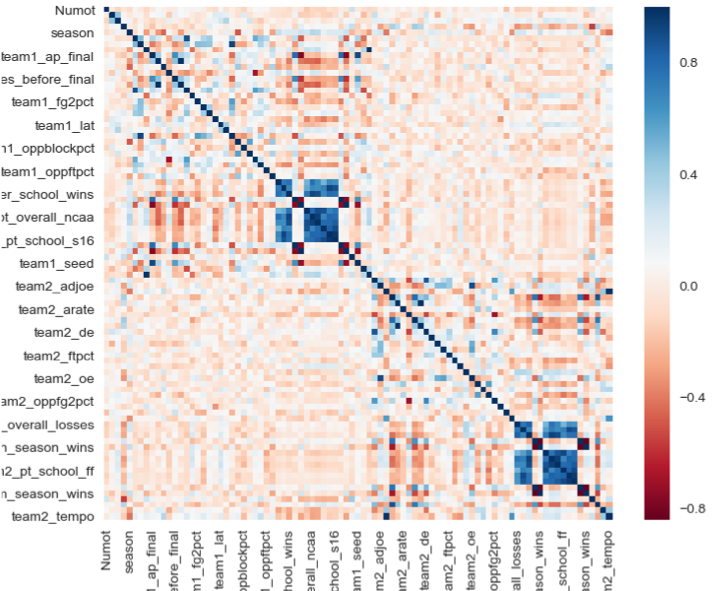
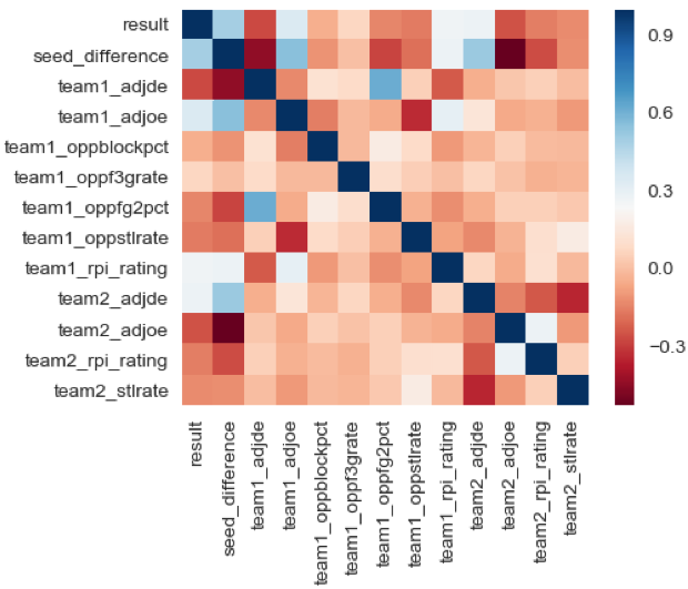
To see the correlation between the game result and all variables. 56 variables – Original data 48 variables – Drop irrelevant variables such as ID, names. Add New Variables 29 variables – Check Multi-collinearity variables transformation
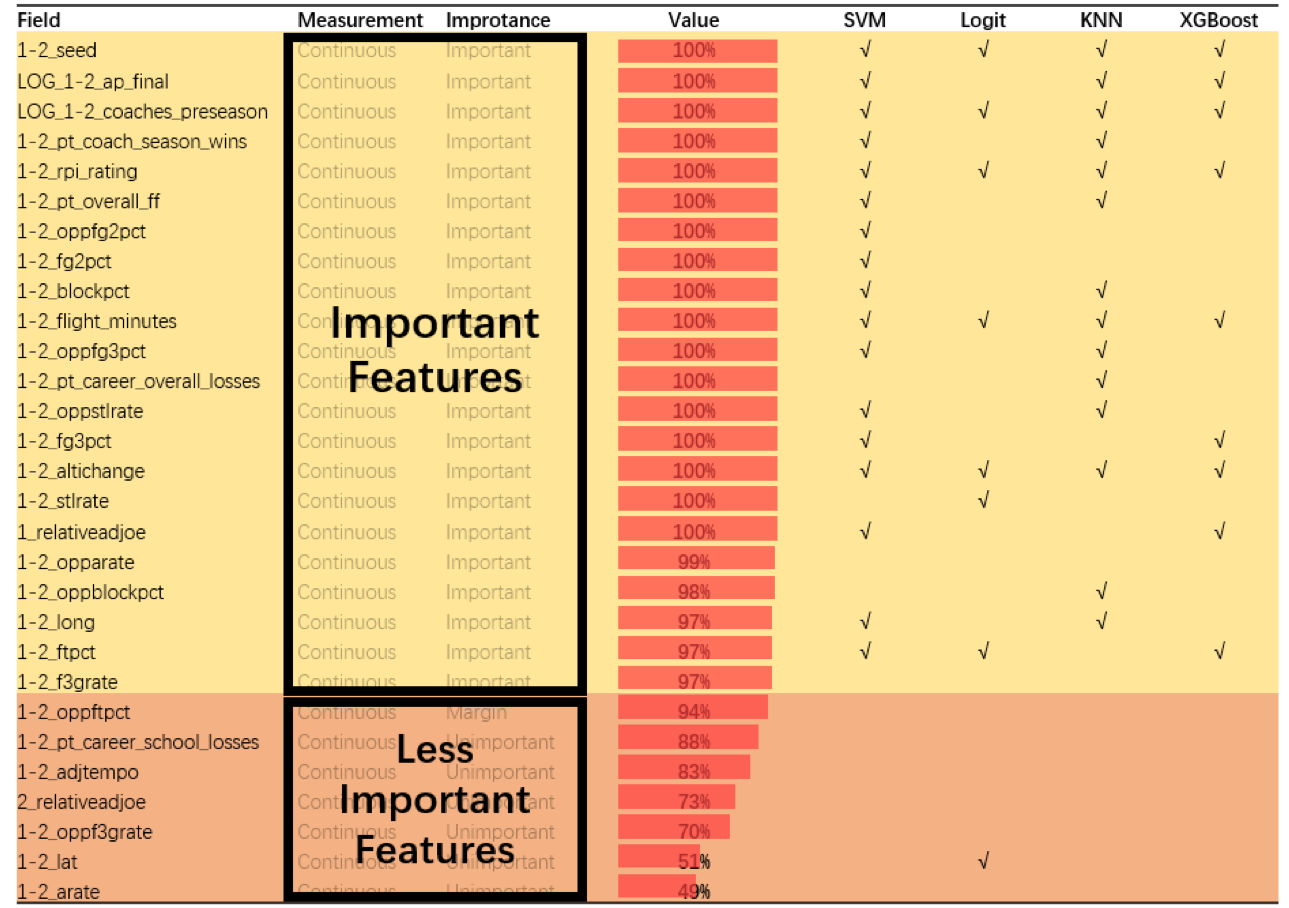
SVM: 17 Variables Logistic: 8 Variables KNN: 14 Variables XG Boost: 9 Variables
- Based on the model’s predictor importance
- Meet model assumptions
- Avoid overfitting
- Features for logistics regression are obtained by forward/backward stepwise, SPSS feature selection, etc.
6 Model Introduction
6.1 KNN(K-Nearest Neighbors)
KNN algorithms classify new data points based on a similarity measures (e.g. distance function). The data is assigned to the class which has the most nearest neighbors.
6.2 XG Boost
Gradient boosting is an approach where new models are created that predict the residuals or errors of prior models and then added together to make the final prediction.
6.3 SVM (Support Vector Machine)
SVM is a discriminative classifier formally defined by a separating hyperplane. Given labeled training data, the algorithm outputs an optimal hyperplane which categorizes new examples.
6.4 Logistic Regression
Logistic Regression is a statistical method for analyzing a dataset with one or more independent variables and binary response.
7 Model Setting
Data Partition into 70% training set and 30% testing set. KNN: K = 7 SVM: SVM kernel type is RBF XG Boost: Learning rate = 0.2, Maximum depth of a tree = 3, Minimum sum of instance Weight needed in a child = 1, Max number of iterations: 20, Learning objective: binary Logistic regression.
8 Model Performance
8.1 Comparison between XG-Boost and Logistic Regression
Repeated tests: 1000 times. In each test, data is randomly partitioned into training and testing set. Accuracy and log-loss are calculated on both sets. Distribution of stats can be found in the histogram.
In the testing set, the two models have a similar performance, however the XG-Boost performs much better in the training set then in the testing set, thus it has a serious overfitting problem. Logit, on the other hand, performs similarly in both training and testing.

8.2 Ultimate Model – Logistic Regression Model
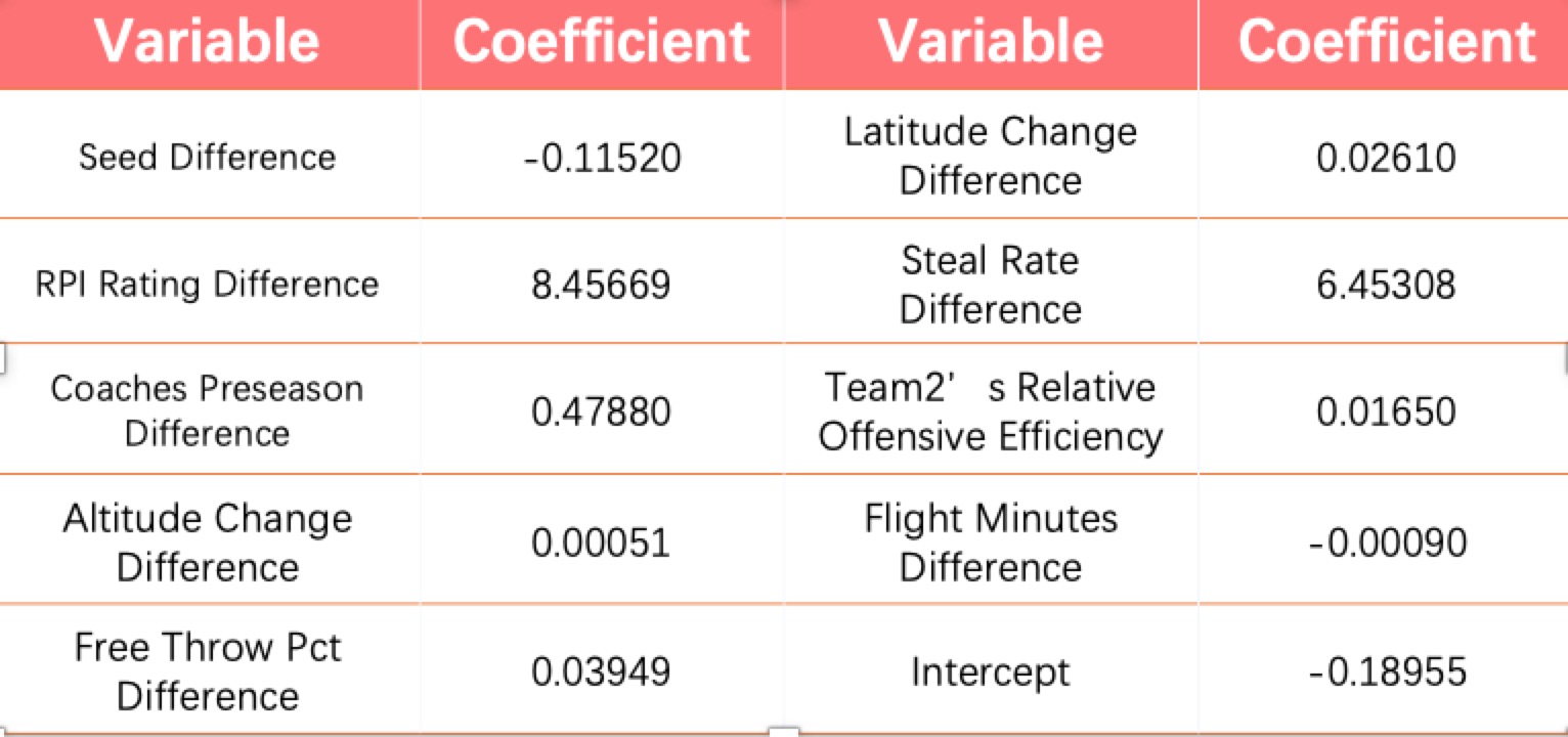
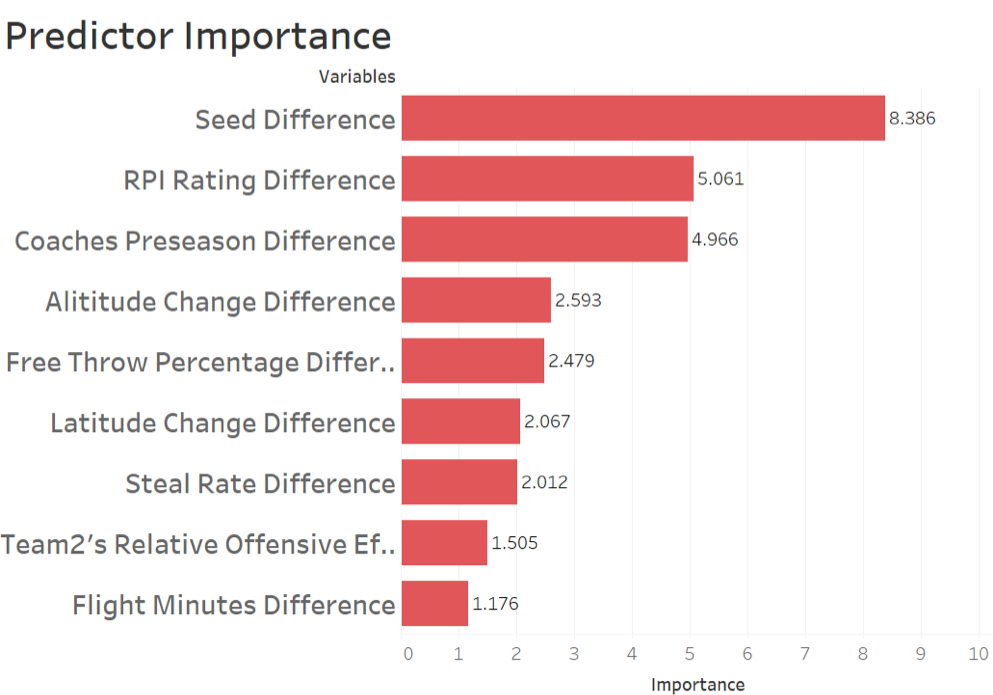
9 predictors were chosen in the ultimate logistic model. The importance of them is shown by the right figure. And the specific parameters are shown below.
9 Conclusion
We tried 4 different models for predicting the winning probability of each game, which are KNN, SVM, Logistic Regression and XG-Boost. Through comparing them according to their performance in log loss and accuracy, we finally chose logistic regression model as our predicting model and gave our predictive probabilities for all the possible games in 2018 Tournament. In order to intensify the predicting model, we perform a series of variables selection to determine the best group of variables to include in our model. Flight time and altitude change, as 2 new variables, were merged into the dataset. We believe they have significant impact on players’ performance. And the result shows that these two variables have quite good performance in our models. In order to get better predicting result, we should focus more on the current status of the team. To be specific, some statistic data like current injuries or pre-competition training level may better indicate the team’s condition before the game, which will surely improve our predicting models.